本文實例講述了Python實現的各種常見分布算法。分享給大家供大家參考,具體如下:
#-*- encoding:utf-8 -*-import numpy as npfrom scipy import statsimport matplotlib.pyplot as plt######################二項分布#####################def test_binom_pmf(): ''' 為離散分布 二項分布的例子:拋擲10次硬幣,恰好兩次正面朝上的概率是多少? ''' n = 10#獨立實驗次數 p = 0.5#每次正面朝上概率 k = np.arange(0,11)#0-10次正面朝上概率 binomial = stats.binom.pmf(k,n,p) print binomial#概率和為1 print sum(binomial) print binomial[2] plt.plot(k, binomial,'o-') plt.title('Binomial: n=%i , p=%.2f' % (n,p),fontsize=15) plt.xlabel('Number of successes') plt.ylabel('Probability of success',fontsize=15) plt.show()def test_binom_rvs(): ''' 為離散分布 使用.rvs函數模擬一個二項隨機變量,其中參數size指定你要進行模擬的次數。我讓Python返回10000個參數為n和p的二項式隨機變量 進行10000次實驗,每次拋10次硬幣,統計有幾次正面朝上,最后統計每次實驗正面朝上的次數 ''' binom_sim = data = stats.binom.rvs(n=10,p=0.3,size=10000) print len(binom_sim) print "mean: %g" % np.mean(binom_sim) print "SD: %g" % np.std(binom_sim,ddof=1) plt.hist(binom_sim,bins=10,normed=True) plt.xlabel('x') plt.ylabel('density') plt.show()######################泊松分布#####################def test_poisson_pmf(): ''' 泊松分布的例子:已知某路口發生事故的比率是每天2次,那么在此處一天內發生4次事故的概率是多少? 泊松分布的輸出是一個數列,包含了發生0次、1次、2次,直到10次事故的概率。 ''' rate = 2 n = np.arange(0,10) y = stats.poisson.pmf(n,rate) print y plt.plot(n, y, 'o-') plt.title('Poisson: rate=%i' % (rate), fontsize=15) plt.xlabel('Number of accidents') plt.ylabel('Probability of number accidents', fontsize=15) plt.show()def test_poisson_rvs(): ''' 模擬1000個服從泊松分布的隨機變量 ''' data = stats.poisson.rvs(mu=2, loc=0, size=1000) print "mean: %g" % np.mean(data) print "SD: %g" % np.std(data, ddof=1) rate = 2 n = np.arange(0,10) y = stats.poisson.rvs(n,rate) print y plt.plot(n, y, 'o-') plt.title('Poisson: rate=%i' % (rate), fontsize=15) plt.xlabel('Number of accidents') plt.ylabel('Probability of number accidents', fontsize=15) plt.show()######################正態分布#####################def test_norm_pmf(): ''' 正態分布是一種連續分布,其函數可以在實線上的任何地方取值。 正態分布由兩個參數描述:分布的平均值μ和方差σ2 。 ''' mu = 0#mean sigma = 1#standard deviation x = np.arange(-5,5,0.1) y = stats.norm.pdf(x,0,1) print y plt.plot(x, y) plt.title('Normal: $/mu$=%.1f, $/sigma^2$=%.1f' % (mu,sigma)) plt.xlabel('x') plt.ylabel('Probability density', fontsize=15) plt.show()######################beta分布#####################def test_beta_pmf(): ''' β分布是一個取值在 [0, 1] 之間的連續分布,它由兩個形態參數α和β的取值所刻畫。 β分布的形狀取決于α和β的值。貝葉斯分析中大量使用了β分布。 ''' a = 0.5# b = 0.5 x = np.arange(0.01,1,0.01) y = stats.norm.pdf(x,a,b) print y plt.plot(x, y) plt.title('Beta: a=%.1f, b=%.1f' % (a,b)) plt.xlabel('x') plt.ylabel('Probability density', fontsize=15) plt.show()######################指數分布(Exponential Distribution)#####################def test_exp(): ''' 指數分布是一種連續概率分布,用于表示獨立隨機事件發生的時間間隔。 比如旅客進入機場的時間間隔、打進客服中心電話的時間間隔、中文維基百科新條目出現的時間間隔等等。 ''' lambd = 0.5# x = np.arange(0,15,0.1) y =lambd * np.exp(-lambd *x) print y plt.plot(x, y) plt.title('Exponential: $/lambda$=%.2f' % (lambd)) plt.xlabel('x') plt.ylabel('Probability density', fontsize=15) plt.show()def test_expon_rvs(): ''' 指數分布下模擬1000個隨機變量。scale參數表示λ的倒數。函數np.std中,參數ddof等于標準偏差除以 $n-1$ 的值。 ''' data = stats.expon.rvs(scale=2, size=1000) print "mean: %g" % np.mean(data) print "SD: %g" % np.std(data, ddof=1) plt.hist(data, bins=20, normed=True) plt.xlim(0,15) plt.title('Simulating Exponential Random Variables') plt.show()test_expon_rvs()
新聞熱點


疑難解答